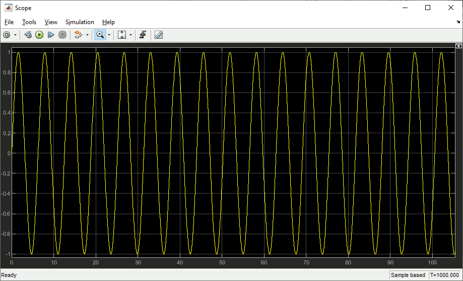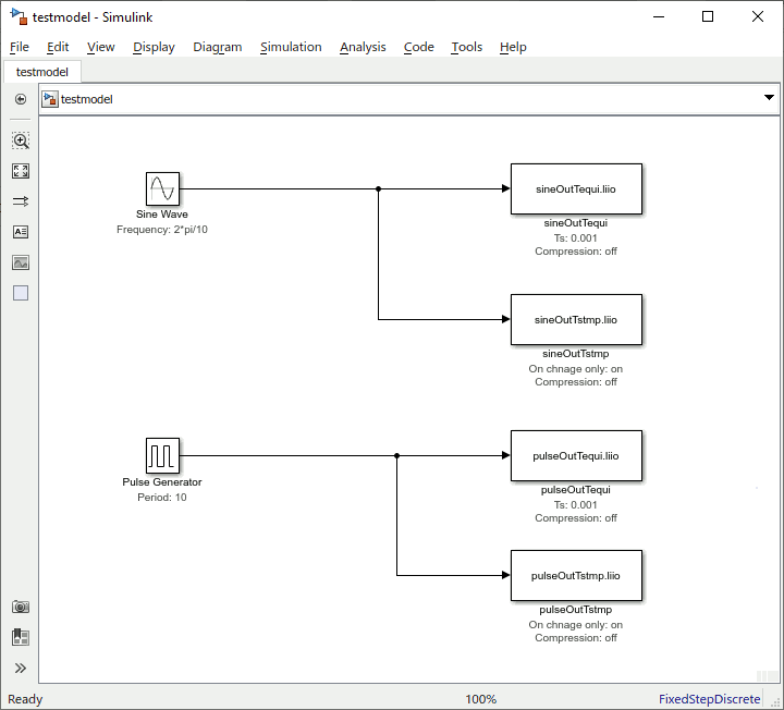
To output a signal to file, you have the choice of the equidistant file-output block liio_sfunouttequi and the time stamped file-output block liio_sfunouttstmp. They both have their pros and cons, as we can see in the following example, where one signal is a continiously changing sine wave signal completing a full wave every 10 seconds, and the other a pulse with the same period of 10 seconds:
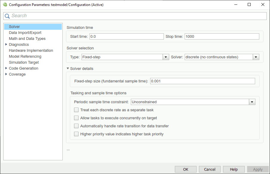
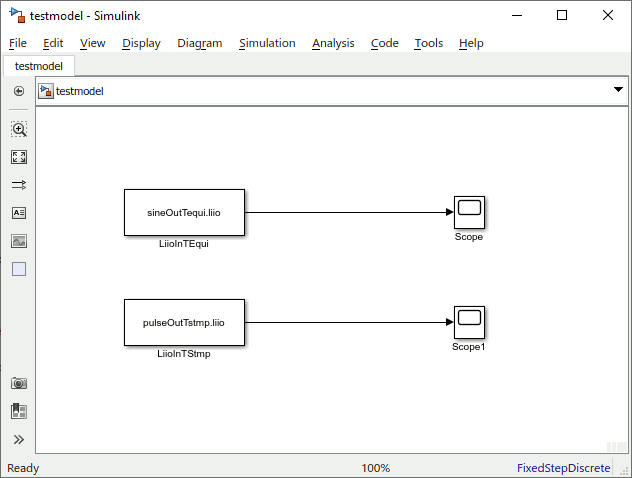
This all discrete example model is set to a respective solver with a sample time of a millisecond and a simulation time of 1000 seconds:
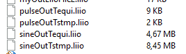
The resulting files quite differ in size:
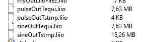
The equidistant output files have both the same size. But for the continiuously changing sine wave the time stamped file has twice the size, as 8 bytes for the scalar double are accomanied by 8 bytes for the time stamp for each and every time step. And for the pulse signal with its rarely changing value its only 0.05% of the equidistant files sizes, as there are only two changes per 10,000 millisecond period, adding up to 2*8*(2*100+1) = 3216 bytes for 100 periods plus the initial value. The rest of the files size is the 512 bytes header.
Using the same model with compression switched on for all file-outputs the result looks like this:
All file sizes are considerably smaller, especially the equidistant pulse signal, as it contains most redundancy. Where the files to be written reside on rather slow devices like classic hard disks or net shares, the execution times of i/o intensive models also drop considerably. But with data written to an internal nvme ssd the compression overhead miht be slightly larger than the time saved by less file data writing effort.
For the example model testing with
tic;sim('testmodel');toc
the time consumption was about 15 sec writting compressed to nvme and 13 sec writting uncompressed to the same device.
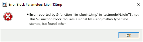
To feed a signal from file to simulation, you have the choice of the equidistant file-input block liio_sfunintequi and the time stamped file-input block liio_sfunintstmp. As already mentioned for the output blocks, they both have their pros and cons with regards to file size and performance. The difference here is that the type of signal storing is already determined by the respective file. So for time stamped files you need to use the time stamped input block, and for equidistant signal data storage the equidistant input block. Inappropriate signal file types will yield an error message like this:
To find out about a .liio-file's properties you can use liio_finfo. Using one of the resulting files of above chapter it looks like:
>> liio_finfo pulseOutTstmp.liio
@@@ Info for LIIO signal file 'pulseOutTstmp.liio':
	File format version: 1.1
	Signal data type: LIIO_DOUBLE_TYPE
	Signal width: 1
	Signal length: 201
	Signal offset: 512
	Compression type: LIIO_COMP_NONE
	Time type: LIIO_TIME_MLSTMP_TYPE
	Fixed step time (0 if stamped): 0.000000
	Start time: 0.000000
	End time: 1000.000000
	ID: 'C:\Users\Robert\Documents\MATLAB\li\liio\pulseOutTstmp.liio'
	Secondary ID: ''
	Tertiary ID: ''
Using two output files from previous chapters example, you can use the input blocks like this:
Yielding retrieved data in the two attached scopes for sine wave (Scope):
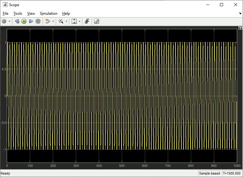
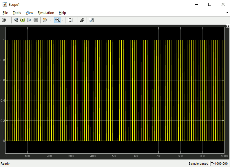
and pulses (Scope1).
In most cases one will not only want to use input data created by LI Buffered File I/O-Blocks in another model. Using liio_write a .liio-file can be created from any data that can be imported to Matlab® variables, or from results of data processing from within Matlab®. In a script or on the command line one might type:
>> t = (0:.001:1000)';
>> x1 = sin(t);
>> liio_write(x1, .001, 'sine', 'sinTequi.liio', false);
>> x2 = double(mod(t, 10) < 0.5);
>> nIdx = [1;find(x2(2:end)~=x2(1:end-1))+1];
>> liio_write(x2(nIdx), t(nIdx), 'pulse', 'pulseTstmp.liio', false);
Here producing from scratch the equidistant sine wave and the time stamped pulse example streamed from model to file in the first chapter and streamed from file to model in the second chapter.
Also signal data stored over simulation to a .liio-file will often require display, analysis or further processing inside or outside of Matlab®. So using function liio_read along the files produced in previous example, signal data might be read to variables and displayed like:
>> [t1, x1] = liio_read('sinTequi.liio');
>> plot(t1, x1);
>> figure;
>> [t2, x2] = liio_read('pulseTstmp.liio');
>> plot(t2, x2);
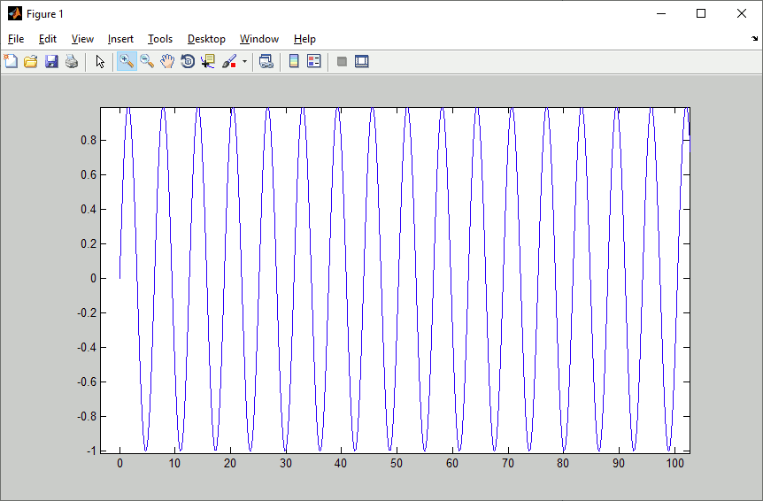
The plotting rersults then should look like this for the sine wave (zoom to first 100 sec):
And like this for the pulse (also zoom to first 100 sec):
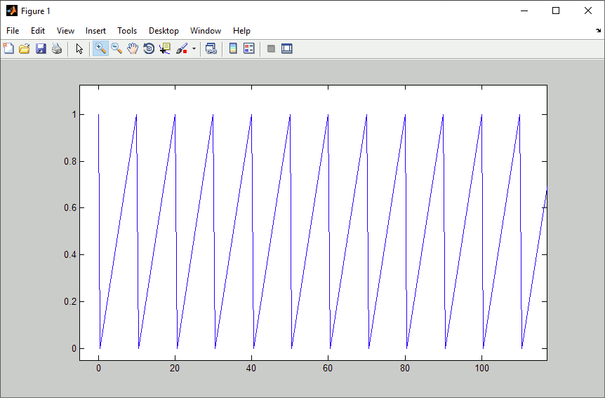
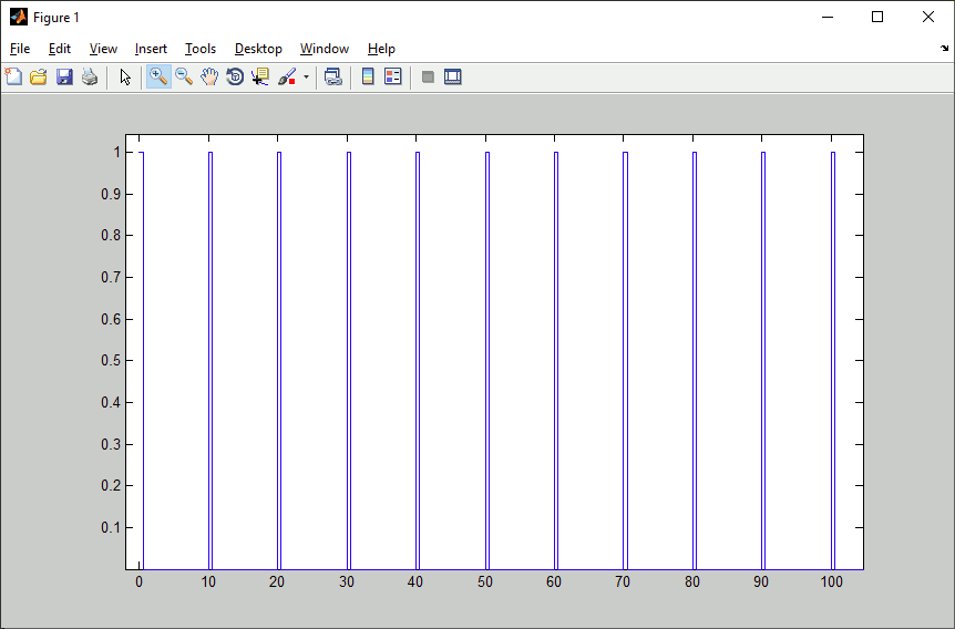
You will notice, that this is a saw tooth rather than the pulse as expected. This is because the time stamped format assumes zero order hold between discrete points on time axis, while the plot applies first order assumption (linear interpolation). Applying zero order hold to a 1 millisecond raster, the result will look like the scope output from Scope1 in chapter 2 again (only zommed to 100 sec):
>> [t_tmp, x_tmp] = liio_read('pulseTstmp.liio');
>> t2 = 0:.001:1000;
>> idx = 1;
>> x2 = nan(size(t2));
>> for k = 1:length(t2)
if idx < length(t_tmp) && t_tmp(idx+1) <= t2(k)
idx = idx + 1;
end
x2(k) = x_tmp(idx);
end
>> plot(t2, x2);
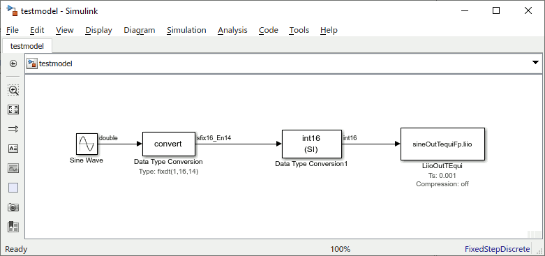
Many Simulink® controller implementations use explicit fixed point signals. But, as in C, the LI Buffered File I/O-Blockset does not come with fixed point information on the basic integer types. To get around this, the solution is relatively easy. The Data Type Conversion block can be set to preserve the stored integer (i.e. the raw value in memory). Like this there is no processing on the signal during simulation, provided there is no difference in the byte length of the integer base.
In analogy to the first two chapters' sine wave examples writing fixed point to .liio-files can be done like this:
And reading fixed point from .liio-files accordingly:
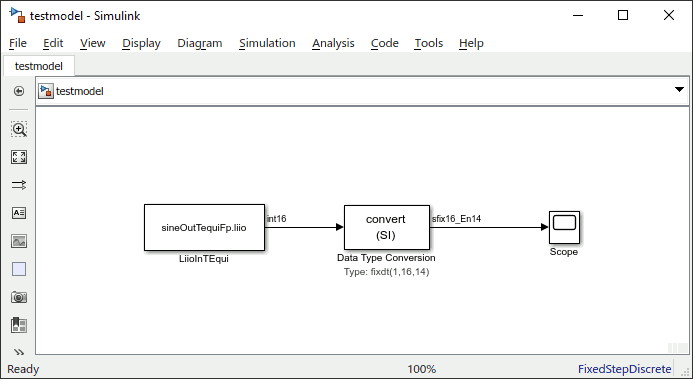
The scope output should then be again (zoomed into first 100 secs):